Use PmPNet to Identify PmP Phase
Build the Running Environment
Note
PmPNet is designed to operate on CUDA with at least 2,100-MiB memory. And Python version is better to choose 3.8.
Assuming you have Anaconda already, set up a new environment named e.g., PmPNet:
conda create -n PmPNet python=3.8
Install JupyterLab or Jupyter Notebook which is used to run PmPNet then:
conda install -c conda-forge jupyterlab
Install pandas to facilitate file manipulations:
pip install wheel
pip install pandas
Install ObsPy which is used to process seismic data then:
conda install -c conda-forge obspy
Install scikit-learn which is used to prepare the train and validation data (e.g., standardization, randomly allocate train and validation data) then:
conda install -c conda-forge scikit-learn
Install pickle-mixin which is used to transform a complex object into a byte stream and speed up data manipulation (e.g., reading and writing) then:
pip install pickle-mixin
Install PyTorch which is used to construct and run PmPNet then:
Note
Be careful about the software compatibility between PyTorch and CUDA.
You can check your CUDA version through nvidia-smi (assume you have installed the NVIDIA Linux driver),
then choose a suitable PyTorch version at https://anaconda.org/pytorch/pytorch/files.
conda install -c pytorch pytorch=1.11.0=py3.8_cuda11.3_cudnn8.2.0_0
Prepare training and validation data
There’re 13 variables (highlighted are must-be variables while others can leave with empty) involved in training and validation data, they’re:
waveform file name: signal_fname = []signal envelope(normalized in the time window from 2s before to 5s after P-wave): envelop_signal = []earthquake ID given by the data center: signal_evid = []
earthquake lontitude: signal_evlo = []
earthquake latitude: signal_evla = []
earthquake depth: PmP_evdp = []earthquake magnitude: PmP_mag = []
station lontitude: signal_stlo = []
station latitude: signal_stla = []
earthquake-station distance: PmP_dist = []PmP label(1, true PmP; 0, false PmP): PmP_label = []PmP arrival time(PmP-P differential traveltime time): PmP_time = []First-P traveltime: PmP_ptime = []
The data can be prepared using python script DataReadin.ipynb.
Train PmPNet
Device configuration, Hyper-parameters setting, paths setting for data and result folders:
import torch
import os
import PmPNet as PN
# Device configuration
cuda = torch.cuda.is_available()
device = torch.device('cuda' if torch.cuda.is_available() else 'cpu')
# Hyper-parameters
batch_size = 200
num_epochs = 80
learning_rate = 1e-3
# Paths for different folders, data and result folders
datadir="/home/pmpboy/Github/Data"
wdir="/home/pmpboy/Github/Result/Train_PN_result"
if not os.path.exists(wdir):
os.makedirs(wdir)
read in the training data:
train_loader, test_loader = PN.readin_data_train(datadir,"TrainData_PmP_Net",batch_size)
train PmPNet:
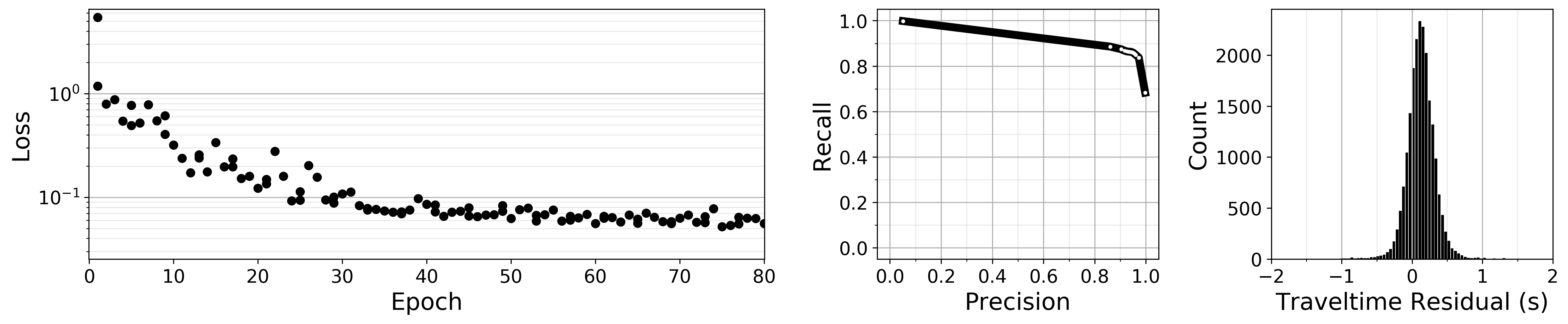
PN.NetTrain(wdir,"train_PN_log","net_PN_model",train_loader,learning_rate,num_epochs,batch_size,device)
We will see such output during training PmPNet:
Epoch [1/80], Step [1/420] Loss1: 3.105050,Loss2: 1.987768,Loss3: 0.338054
Epoch [1/80], Step [101/420] Loss1: 0.527436,Loss2: 0.298014,Loss3: 0.143794
Epoch [1/80], Step [201/420] Loss1: 0.458504,Loss2: 0.414377,Loss3: 0.150728
Epoch [1/80], Step [301/420] Loss1: 0.396632,Loss2: 0.524836,Loss3: 0.144453
Epoch [1/80], Step [401/420] Loss1: 0.355758,Loss2: 0.687848,Loss3: 0.141200
Epoch [2/80], Step [1/420] Loss1: 0.371204,Loss2: 0.692910,Loss3: 0.128348
Epoch [2/80], Step [101/420] Loss1: 0.386219,Loss2: 0.625399,Loss3: 0.130919
Epoch [2/80], Step [201/420] Loss1: 0.307851,Loss2: 0.350751,Loss3: 0.122441
Epoch [2/80], Step [301/420] Loss1: 0.273838,Loss2: 0.373369,Loss3: 0.145047
Epoch [2/80], Step [401/420] Loss1: 0.279507,Loss2: 0.928377,Loss3: 0.130401
Epoch [3/80], Step [1/420] Loss1: 0.264289,Loss2: 0.560267,Loss3: 0.149387
Epoch [3/80], Step [101/420] Loss1: 0.269108,Loss2: 0.351606,Loss3: 0.130983
......
model evaluation on test data:
PN.netevalu(wdir,"net_PN_model","prcurve_file","predict_PN_file",test_loader,device)
quickly visualize the result:
PN.plot_modeva(wdir,"train_PN_log","prcurve_file","predict_PN_file","plot_PN_modevalu")
Apply the pre-trained PmPNet to a certain year data
read in the real data:
test_loader = PN.readin_data_real(datadir,"ValidationData_2015",batch_size)
predict probability the waveform contains a clear PmP phase and PmP traveltime:
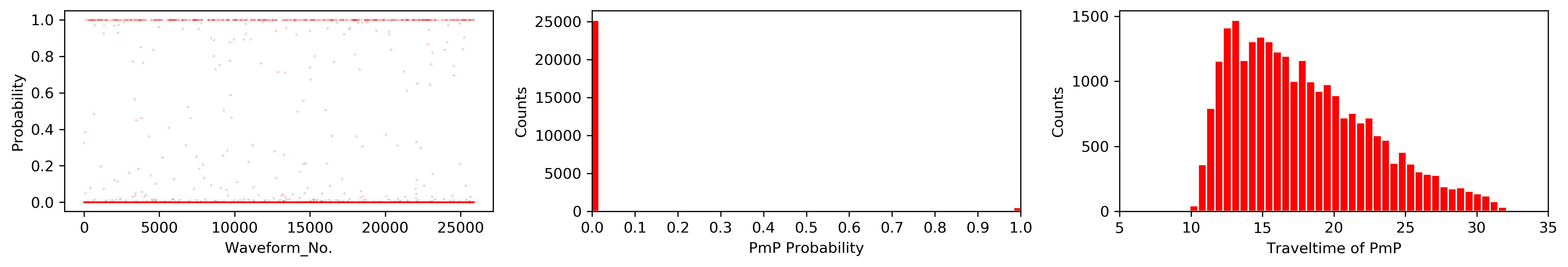
PN.netpredict(datadir,"ValidationData_2015",wdir,"net_PN_model","predict_PN_file_2015",test_loader,device)
We will see such output during the process:
NO.: 0   ID: 37272439   PmP_Prob: 0.323879  PmP_Time: 20.893116  dist: 127.9   evdp: 11.59   mag: 2.1  evtnm: 20151113_1204.CI.DTP
NO.: 1   ID: 37198399   PmP_Prob: 0.000000  PmP_Time: 17.361309  dist: 103.3   evdp: 18.04   mag: 2.3  evtnm: 20150705_1315.CI.SYN
NO.: 2   ID: 37150703   PmP_Prob: 0.000001  PmP_Time: 14.302899  dist: 76.6   evdp: 6.28   mag: 2.4  evtnm: 20150423_1454.CI.TOR
NO.: 3   ID: 37501608   PmP_Prob: 0.000037  PmP_Time: 13.073999  dist: 60.6   evdp: 2.31   mag: 2.2  evtnm: 20151214_0708.CI.DPP
NO.: 4   ID: 37508080   PmP_Prob: 0.000002  PmP_Time: 19.669258  dist: 111.8   evdp: 2.76   mag: 2.3  evtnm: 20151230_1027.CI.JVA
NO.: 5   ID: 37148391   PmP_Prob: 0.000000  PmP_Time: 16.840071  dist: 91.2   evdp: -0.18   mag: 2.3  evtnm: 20150420_0231.CI.HEC
NO.: 6   ID: 37305208   PmP_Prob: 0.000026  PmP_Time: 24.993418  dist: 151.4   evdp: 6.62   mag: 2.5  evtnm: 20150114_1203.CI.SYP
NO.: 7   ID: 37301936   PmP_Prob: 0.000000  PmP_Time: 26.983143  dist: 170.9   evdp: 8.30   mag: 2.5  evtnm: 20150104_0943.CI.GATR
NO.: 8   ID: 37402872   PmP_Prob: 0.000000  PmP_Time: 18.354214  dist: 102.4   evdp: 2.52   mag: 2.5  evtnm: 20150618_1256.CI.BLC
NO.: 9   ID: 37403528   PmP_Prob: 0.000005  PmP_Time: 19.624937  dist: 111.2   evdp: 1.40   mag: 2.2  evtnm: 20150619_0218.CI.RVR
......
quickly visualize the result:
PN.plot_modpredict(wdir,"predict_PN_file_2015","plot_PN_predict2015")